Other Examples
3.1 Problem
You would likely come across randomness outside of the statistics classroom when learning about, for example, genetic drift or mutations (biology; Martin & Hine, 2008), radioactivity or lasers (physics; Daintith, 2009), dispersion (geology; Allaby, 2013), and diffusion (chemistry; Daintith, 2008), as well as when conducting research (Gougis et al, 2017). How these subjects consider randomness could contribute to our understanding of the concept. In particular, the use of randomness in subjects other than statistics demonstrates real-world examples where random phenomena may be encountered.
Expanding on lexical ambiguity as a potential source of randomness misconceptions, it is feasible that a lack of consistency between school subjects could also be a potential source of randomness misconceptions.
Learning Aims:
- Explore and discuss everyday examples using the previous skills attained in the definition and distribution sections.
- Investigate the genetic randomness of Huntington’s Disease.
- Explore diffusion as an example of randomness in chemistry with connections to sample size and fluctuations about the mean.
- Consider how random events build into a distribution with a radioactive decay example.
3.2 Everyday Examples
There are so many everyday examples of randomness - check out one (or many) that interest you from the options below!
Coffee Shop
You are observing customers entering a coffee shop between 10 am and 11 am one day. You record how long it took for the door to open since the last customer entered. Every time the door opens, this counts as one “event” and we will assume only one person enters.

You obtain the following dot plot of waiting times:

How could we represent this data in other ways?
|
|
|
|
|
|
- What did you like about each example?
- What did you dislike?
- Did all of the examples represent the data?
Run a simulation!
- What distribution will you use in Scampy?
- What will be the rate? (Use 1/mean, i.e., 1 event per “mean” minutes)
- What will you change the units to?
- What kind of distribution did it create?
- What time interval will you specify for the Distribution of Counts?
- Imagine what the fuzz might look like if we repeated the simulation many times. Do you think the distribution you used works well for this example?
Roulette
At a visit to the casino, a friend bets $20 on “black” at the roulette table. They did not consider what events had previously occurred before placing their bet, they just picked black and went for it!

Your other friend at the casino saw that the last five numbers to come up were all red. “It’s a run of reds” they whisper to you, before placing a $20 bet on red.
A man sitting at the roulette table hands you a piece of paper. “Here are the last 30 numbers to come up…”

Earthquakes
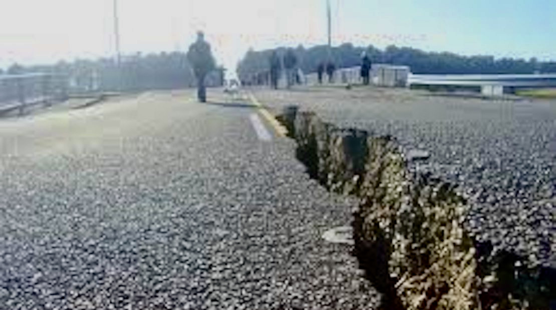
Geonet.org.nz identify around 20,000 earthquakes (rū) in New Zealand every year - although most are too small or too deep for most people to notice. Generally, we expect approximately 3 strong earthquakes every 2 years (magnitude 6.0-6.9) and 1 very strong earthquake every 4 years (magnitude 7.0-7.9).
The following is a plot of the earthquakes in New Zealand that were above magnitude 6.0:
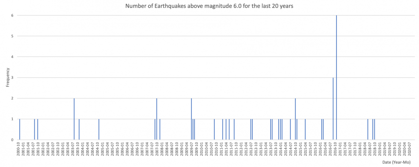
The following depicts the waiting times between earthquakes in New Zealand that were above magnitude 6.0:

It has been over 700 days since New Zealand last recorded a magnitude 6.0+ earthquake.
- How long do you estimate it to be until the next magnitude 6.0+ earthquake occurs in New Zealand? (You may provide a range of days if you like)
- How confident are you with your estimate for how many days it might be until the next magnitude 6.0+ earthquake occurs in New Zealand?
Let’s explore some more!
- Open up Scampy and head to the Simulation tab. Set the distribution to exponential and the rate as 0.25 (i.e. 1 very strong earthquake every 4 years). Set the units as “years”. Run the simulation and, when you get to the Distribution of Counts, set an appropriate time interval (i.e., 1 year).
- What do you think? What was the smallest waiting time? What was the largest? How confident are you in your previous estimate now?
Community Time!
In this example, Earthquakes, we learnt about how earthquakes can be unpredictable.
Ask your community about their experiences with earthquakes. Do you know anyone who experienced the Christchurch earthquake in 2010?
Volcanos

Think about the occurrence of volcanic eruptions (hūnga). Suppose a particular volcano is thought to erupt once every 200 years. What might the occurrence of these eruptions look like over 2000 years?
On a piece of paper, draw a timeline from year 0 to year 2000 (I recommend making the line 20 centimetres long and adding 200 years every 2cm). Then add on your volcanic events!
- What did you first consider once your timeline was drawn?
- Did you calculate anything before placing the events?
- Did you need to work anything out?
In New Zealand, we have had four volcanic eruptions since 2000 - most recently in 2019.
This plot shows the occurrence of volcanic eruptions since 1845 (there have been 11).

The average waiting time between eruptions is 15.7 years.
Which of the following options depict the waiting times between volcanic eruptions in New Zealand?
|
|
|
|
|
|
- What do you think? What was the smallest waiting time? What was the largest?
- Which of the options was most intuitive?
- Which of the options made the waiting times most clear?
- Can you think of some pro’s and con’s for each option? What did you like or dislike about each one?
Community Time!
In this example, Volcanos, we learnt about how volcanic eruptions can be unpredictable.
Ask your community about their experiences with volcanic eruptions. Do you know anyone who has seen a volcano erupting?
Blinks
Think about someone blinking (kamo).
- Are blinks random? Can you predict when someone will blink? What might effect when someone blinks?

We are going to have a play with video mode using the Scampy tool.
This part of the tool allows the user to upload a video of their choice. As we are thinking about blinking, you might like to download the following clip of Barack Obama giving one of his weekly presidential updates back in 2015. Download here.
Otherwise, you could find your own video on Youtube and copy/paste the link into Scampy.
Then, once you have your video, hit play and click to record when someone blink (i.e. every time Obama blinks, hit the click me! button to record the event). Carry on through the Scampy tool and see what data you have collected!
- What kind of distribution do you think will best fit the sample of waiting times generated between each of the blinks you recorded?
Heights

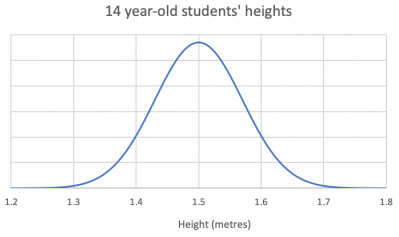
Think about the heights (tāroaroa) of 14-year-olds and what a random sample might look like.
In this class, the students are going to draw a random sample of 20 observations relating to heights. Below shows the distribution of heights of 1,000 14-year-old students:
Which of the following samples best fits your expectation of what a sample of heights might look like?

|

|

|

|
- Which one of the samples from the heights example is least random?
Have a go using data cards in your class! This is a great way of having a go at sampling and noticing the randomness present in each sample drawn. Can you predict what height will be drawn next?
3.3 Biology
Randomness can occur in biological systems. In biology (mātauranga koiora), you might encounter randomness when exploring mutations or cell division, among other areas.
One example of a randomness in biology can be seen in Huntington’s disease. This rare disease is caused by an error in DNA, a defect in a single gene. The disease causes nerve cells in the brain to break down, affecting the patient’s movement, cognition, and psychiatric health. Huntington’s disease has what is known as an “autosomal dominant inheritance pattern”. This means if you have just one copy of this gene, you would likely be affected by the disease.
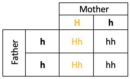
You inherit two copies of genes from your parents (one from each). This means that if one of your parents has Huntington’s, there is a 50% chance that each of their children inherits the disease. In the table, below, H is the Huntington’s Disease gene (with h as a normal gene) and we can see that the output of the punnet square results in a 50% chance of the child inheriting the disease.
We are going to explore the randomness involved in this.
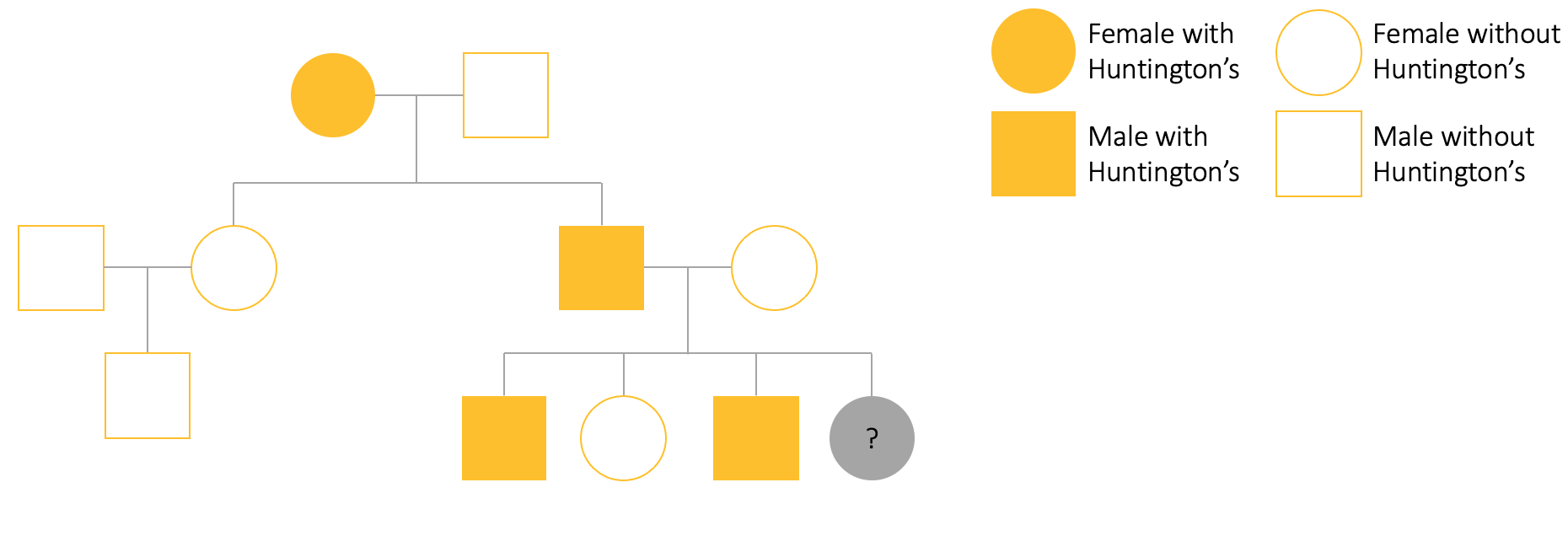
Consider the following pedigree tree for your friend, Sarah. We can see that Granny Salt had Huntington’s disease and this was passed onto one of her children. Aunty Sally did not get the Huntington’s gene but Sarah’s dad, Scott, did. Sarah is the youngest of her siblings and does not know if she has the disease or not. Her family know that both of Sarah’s older brothers have Huntington’s but her sister does not.
3.4 Chemistry
Randomness is a key property the universe. As chemistry (mātai matū) examines the building blocks of the universe, we typically have to deal with this random behaviour. For example, particles are known to move randomly.
One example of this is the movement of gas particles through a semi-permeable membrane. The movement from high to low concentration is not a one-step process - the gas particles continually move around, swapping which side of the membrane they are on. The movement from high to low concentration effects the degree of movement; thinking statistically, if there are more particles on one side of the membrane there will be more movement simply because there are more particles to move!
Let’s visualise this!
To be able to make this example visible, we will need to make some assumptions. Suppose we can observe 4 gas particles in a vacuum chamber set-up. These particles would be moving quickly and randomly. There would continually be a chance that a particular particle crosses the membrane. But, we would have difficulty visualising this! So, let’s assume that we observe the particles during short intervals (2.5 seconds), during which time, each of the particles we are observing have a 50% chance of crossing the membrane.
In the video, we watch the four gas molecules for 25 seconds. During this time, we watch them swap or stay 10 times. Even though the video has some short pauses between each short interval (of 2.5 seconds), this would not be the case in actuality - it is just a consequence of making the video!
We should explore the movement more carefully. In particular, remember how I said “if there are more particles on one side of the membrane there will be more movement simply because there are more particles to move”? This is what we will investigate in more detail.
You could do this activity at home or in class using coins and/or a computer.
Collect as many coins (uka) as you can! Let’s start off with 10 coins and then add some more. Place 8 coins in one pile on the left and the last 2 coins in another pile of the right.
Flip all of the coins in the pile on the left. Place them into “move” and “stay” groups, where a coin is in the “move” group if it is a head and the “stay” group if it is a tail. These coins represent the gas molecules that “start” on the left side of the chemistry experiment set-up - there is a 50% chance they move to the right side and 50% chance they stay on the left side.
- How many coins in the left pile moved? How many stayed?
Do the same with the coins on the right. You should end up with something that looks like this:
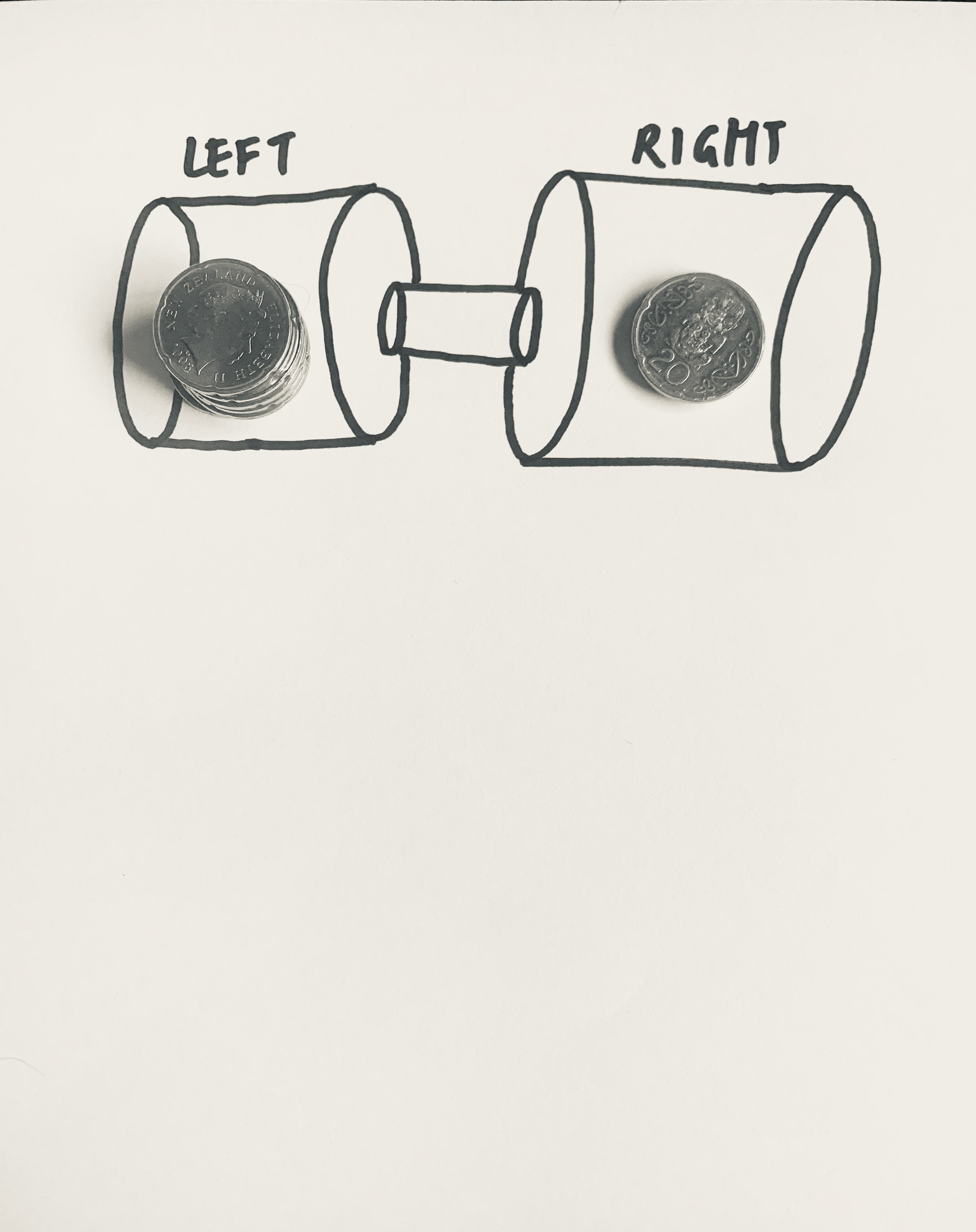
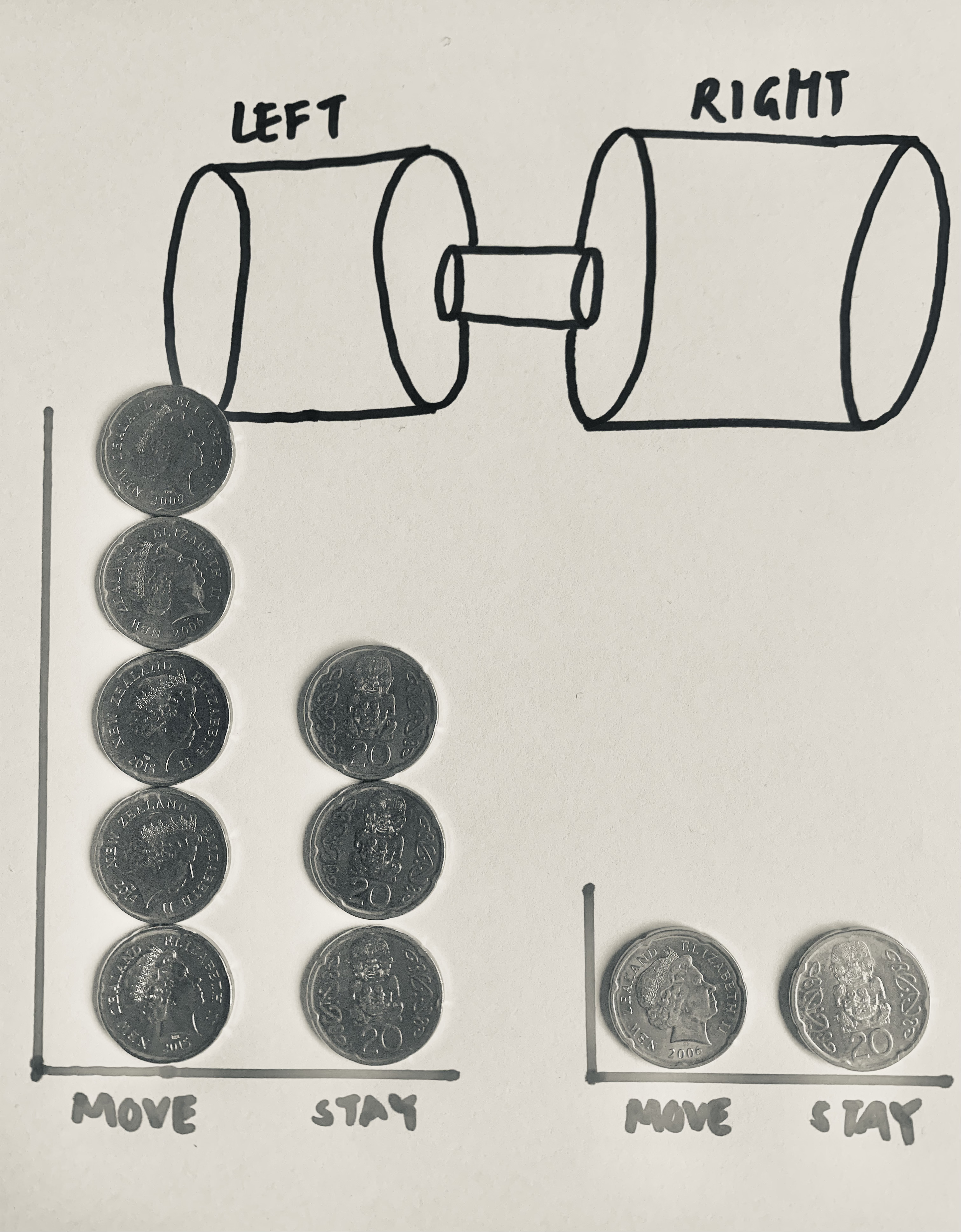
In this example, 62.5% (5/8) moved from the left pile while 50% (2/4) moved from the right pile. After this move, we would have 7 coins in the right pile and 5 coins in the left pile. Relating back to our chemistry example, there was more movement to the side with less molecules!
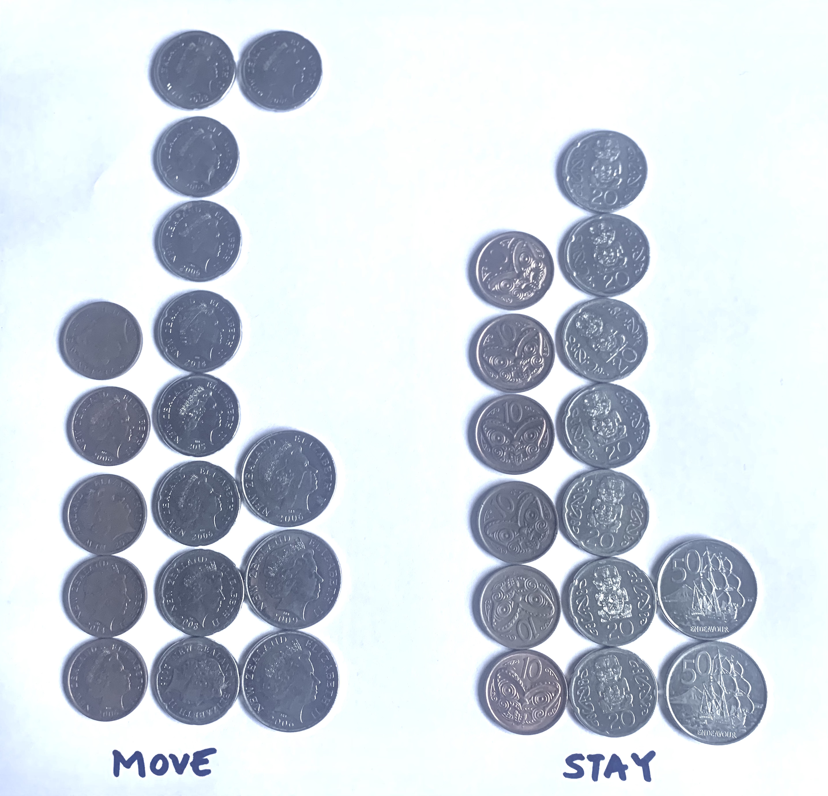
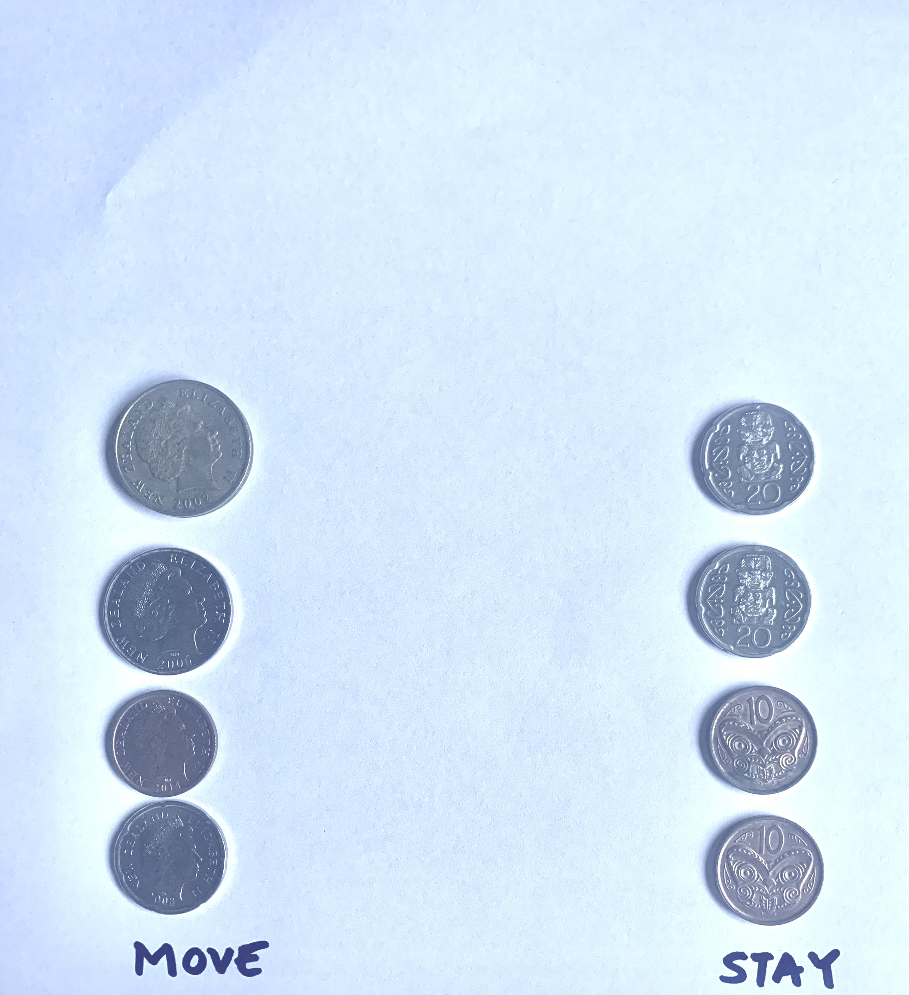
Now, find all the coins you can! Work out what 20% is for how many coins you have found (i.e. I found 40 coins so 20% is 8 coins) and put these in the pile on the right. The rest make a pile on the left. Repeat the steps of flipping the coins and organising them as “move” (heads) or “stay” (tails).
You should end up with something that looks like this. Note, the coins do not hold any value in this example ($2 represents the same as 10c):
| Left Pile | Right Pile |
|
|
This time, 53.125% (17/32) moved from the left pile while, just by chance, 50% (4/8) moved from the right pile. After this move, we would have 21 coins in the right pile and 19 coins in the left pile. Again, there was more movement to the side with less molecules!
Okay, we know there are a lot more gas molecules in our chemistry experiment than what we can represent with coins! So, let’s use some code to increase our sample size (n = number of molecules, in this case).
#Set the number of molecules in each pile and specify our coin toss outcomes
left = 800
right = 200
coin = c('heads: move', 'tails: stay')

#Randomly sample (i.e., do the coin toss!) for each pile and show the first few outcomes (not all 1000!) along with the overall totals
leftPile = sample(coin, size = left, replace = TRUE); head(leftPile); table(leftPile)
## [1] "heads: move" "heads: move" "tails: stay" "heads: move" "heads: move"
## [6] "tails: stay"## leftPile
## heads: move tails: stay
## 392 408rightPile = sample(coin, size = right, replace = TRUE); head(rightPile); table(rightPile)## [1] "heads: move" "heads: move" "heads: move" "heads: move" "tails: stay"
## [6] "tails: stay"## rightPile
## heads: move tails: stay
## 113 87#Calculate the new number of molecules on the left and right
newRight = length(which(leftPile == "heads: move")) + length(which(rightPile == "tails: stay")); newRight## [1] 479newLeft = length(which(leftPile == "tails: stay")) + length(which(rightPile == "heads: move")); newLeft## [1] 521Even if both sides have a move/stay ratio of 50:50, more on one side means the exchange will be greater in one direction than the other (more movement from the larger side).
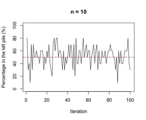
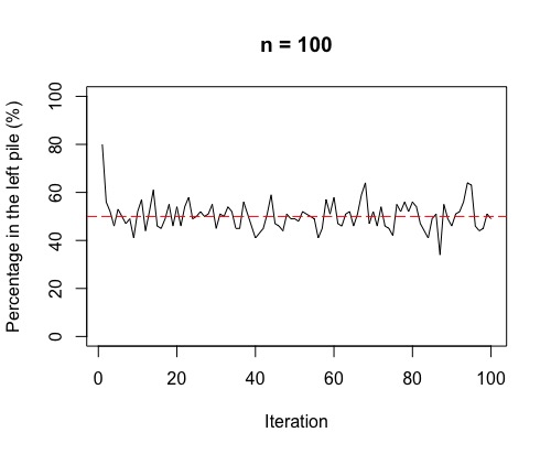
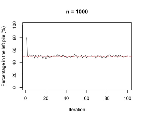
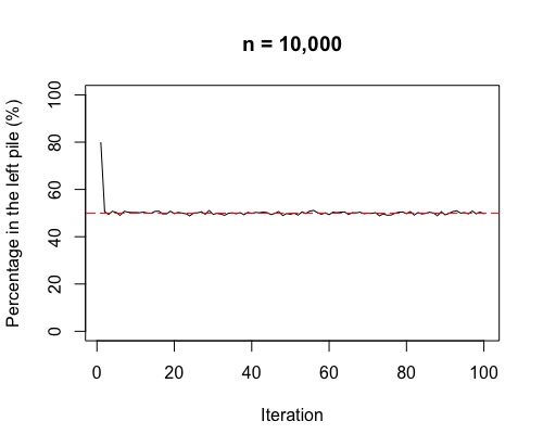
Right, there is one more thing to check out! Often, in chemistry, we think of the movement from high concentration to low concentration across a semi-permeable membrane as being a one-step process. What we see if we run the above simulation 100 times, is a fluctuation around 50%. This fluctuation is more volatile for smaller sample sizes (i.e. few molecules overall).
|
|
|
|
So, as in the plots, the more molecules (or coins in the simulation), the more stable around 50% either side of the membrane (or in each pile for the simulation). If we have a lot of gas molecules, the balance of 50:50 is often quite quick – but, that doesn’t mean there isn’t lots of random movement still! The gas molecules swap sides of the membrane continually and randomly.
3.5 Physics
There are many examples in physics (mātai ahupūngao) where randomness plays a part. One such example is radioactive decay. Do you recall the waiting time Twitter examples in the Distributions tab? This is similar!
Radioactive decay, also known as radioactivity, is where an unstable atom (such as uranium) loses energy through radiation. This is a random process but the decay rate is usually known.
The trouble is, while we know the probability of this occurring, it is impossible to predict which atoms will do so! Sounds familiar, right? This fits to the New Zealand mathematics and statistics curriculum definition!
So, let’s say we have 50 atoms we are watching and the rate of decay is 0.167 atoms every hour.
In the first hour, how many atoms do you expect to decay?
8.33 but, we can’t have a third of an atom! So, let’s say 8 or 9.
Now, this is only in theory so let’s simulate this!
Let’s give it a go! Here are the results of rolling 50 dice. Count how many are a 6.
## [1] "6, 4, 4, 3, 5, 6, 6, 5, 3, 4, 3, 6, 5, 6, 2, 1, 6, 1, 4, 5, 2, 5, 4, 4, 1, 1, 2, 2, 6, 2, 3, 5, 2, 1, 4, 4, 5, 5, 5, 3, 2, 3, 5, 4, 1, 2, 1, 1, 1, 3"There are: 7! So, that means 7 atoms decayed in the first hour.
How many atoms are left? 43!
So, let’s roll for the next hour!
## [1] "1, 2, 1, 5, 3, 5, 1, 2, 2, 2, 6, 1, 2, 3, 2, 2, 2, 4, 6, 2, 4, 2, 5, 1, 1, 2, 5, 3, 6, 3, 6, 1, 4, 5, 2, 3, 5, 1, 3, 5, 3, 1, 6"How many atoms decayed this hour? 5!
We repeat this until there are no more atoms left! If everyone in your class did this activity and you combined your plots, we would get something that looks like this:
This site has been created as part of my PhD thesis on perceptions of randomness. I am always keen for feedback, so please email me any thoughts you have via amy.renelle@auckland.ac.nz. Thank you to my supervisors, Dr. Stephanie Budgett and Dr. Rhys Jones, for their guidance throughout my project. I would also like to thank Anna Fergusson for her help inspiring and creating this website. You can find the references for this site here.